Entanglement

Two degrees of freedom are entangled when the system density matrix cannot be expressed as a mixture of separable states. Besides their fundamental interest, entangled states are highly sought for applications in quantum information processing. Many such implementations might involve QDs as building blocks, as that of Awschalom et al. (2002) or Imamoglu (1999). In the following we consider the possibilities open to the system under consideration.

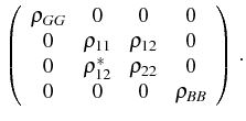
From the couplings that Eq. (6.9) establishes between the different levels in the local basis, it follows that the reduced density matrix for the QDs in the steady state takes the form:

$\displaystyle \rho_\mathrm{QD}^\mathrm{SS}$

$\displaystyle =$

$\displaystyle \left( \begin{array}{cccc} \rho_{GG} & 0 & 0 & 0 \\ 0 & \rho_{11... ...0 & \rho^*_{12} & \rho_{22} & 0 \\ 0 & 0 & 0 & \rho_{BB}\end{array} \right)\,.$

(6.10)

Therefore, the only way to entangle the two dots is to populate the Dicke states $\ket{\mathrm{T}_0/\mathrm{S}}$ (which are two of the so-called Bell states). In a bipartite four-level system, the degree of entanglement can be quantified by the tangle ( $\tau$ ), which ranges from 0 (separable states) to 1 (maximally entangled states) [see the work by Wootters (1998)]. In order to compute $\tau$ , we need to introduce the intermediate quantities and , defined as:

$\displaystyle {T} = \left( \begin{array}{cccc} 0 & 0 & 0 & -1 \\ 0 & 0 & 1 & 0 ... ...right)\quad\mathrm{and}\quad R = \rho_\mathrm{QD} {T} \rho_\mathrm{QD}^* {T}\,.$

(6.11)

The tangle is then

$\displaystyle \tau =[\mathrm{max}\{0,\sqrt{\lambda_1}- \sqrt{\lambda_2}-\sqrt{\lambda_3}- \sqrt{\lambda_4}\}]^2$

(6.12)

where $\{\lambda_1, \lambda_2, \lambda_3, \lambda_4 \}$ are the eigenvalues of

in decreasing order. One finds that whenever it is not zero, the tangle is given by:

$\displaystyle \tau=4(\vert\rho_{12}\vert-\sqrt{\rho_{GG}\rho_{BB}})^2\,.$

(6.13)

We are interested in conditions that maximize $\tau$ : these correspond to large values of the off-diagonal elements $\vert\rho_{12}\vert$ and small populations of the states $\ket{G}, \ket{B}$ . Here, dissipation and pumping cause $\rho_\mathrm{QD}(t)$ to evolve into a mixture, with reduced coherences and nonzero occupancy of all levels. This limits the maximum tangle that can be achieved as was described by Munro et al. (2001). In order to isolate the contribution of such effect, we quantify the degree of purity of the QD states, by computing the linear entropy:

$\displaystyle S_L=\frac{4}{3}[1 - \Tr{( \rho_\mathrm{QD}^2)}]=\frac{4}{3}[1 - \... ...G}^2 +\rho_{11}^2 +\rho_{22}^2 + \rho_{BB}^2 + 2\vert\rho_{12}\vert^2 \big)]\,,$

(6.14)

which is 0 for a pure state, and 1 for a maximally disordered state (where the four dot states have the same probability

**Figure 6.4:** Mean number of photons $\langle n\rangle$ stored in the cavity as a function of the coupling of the second dot , for $\gamma_a=g_1$ , $\Delta_1=\Delta_2=0$ and (all in units of ). Both the cases of independent pumping only (red line, corresponding to $P_\mathrm{ind}=P$ , $P_\mathrm{com}=0$ ) and common pumping only (black and blue lines, with $P_\mathrm{ind}=0$ , $P_\mathrm{com}=P$ ), are plotted. In the latter case, the black line corresponds to $\gamma=0$ and the blue one to $\gamma=5\times10^{-3}g_1$ . Inset: Population of the singlet state. In both plots, the black line has a discontinuity at . The singular value assumed by $\langle n\rangle$ and the singlet population in this case is marked by the black point.
$\includegraphics[width=0.6\linewidth]{chap6/fig_3.ps}$

The entangling of the dots in the singlet state (rather than the triplet) is a natural way to achieve a good degree of tangle and purity at the same time, as in the limiting case where parameters for each dot are identical (, $\Delta_1=\Delta_2$ ), the singlet becomes a ``dark state''. In the case where $P_\mathrm{ind}=0$ , it is also decoherence free [Lidar et al. (1998)], i.e., is not affected by the decoherence introduced by the pump. When the limiting case is only approached ( $g_1 \simeq g_2$ ), $\ket{\mathrm{S}}$ becomes coupled to the triplet-subspace by a small effective coefficient $\delta g$ (see Fig. 6.2), and the population can be trapped in the singlet state (see below). As we already mentioned, equivalent trapping mechanisms have been reported when interacting with a common squeezed bath by Ficek & (2002) and Akram et al. (2000). Our proposal for achieving a high value of the tangle is based on a slight imbalance between the coupling strengths of the QDs, resulting in a very high occupation of the singlet state.

In Fig. 6.4 we plot the mean number of photons and the population of the singlet state (inset), for $\Delta_i=0$ . The first dot is in the strong coupling regime with the cavity ( $\gamma_a / g_1 < 4$ ), whereas the second one goes from weak to strong coupling regime as a function of . If the QDs are pumped independently (red line), the photon number increases with , until the maximum is reached for . The presence of the second dot in strong interaction with the cavity increases nonlinearly the emission (see below).

**Figure 6.5:** Tangle $\tau$ for various detunings, as a function of $P_\mathrm{com}$ (in units of ). Parameters: $\gamma_a=g_1$ , $\gamma=5\times10^{-3}g_1$ , $P_\mathrm{ind}=0$ , . The maximum tangle achieved grows with the detuning but requires a larger pumping.
$\includegraphics[width=0.56\linewidth]{chap6/fig_4.ps}$

On the other hand, when the pump is common, a very different behavior is observed (blue line in Fig. 6.4). First, for , the single-QD limit is not recovered, since the cross pumping term $P_\mathrm{com}$ creates an effective coupling between the QDs, which induces correlation between their states even when no cavity-induced coupling is present. The other striking difference occurs for $\vert g_2-g_1\vert\approx0$ : the photon number decreases, while the singlet population increases. Here, $\delta g \ll g$ , and the singlet is almost decoupled from the dynamics (see Fig. 6.2 and the above discussion). There is a slow flow of population into the singlet state with zero photons, which also has a very long relaxation time. In the specific case , there is an abrupt change of the photon number, and the system turns into an effective three-level system, as the singlet is optically dark.

The strong differences between the emission of a system under independent or common pumping evidenced in Fig. 6.4 (especially when one of the dots is not coupled to the cavity or when they are coupled in a similar way) provide a simple experimental hint to discriminate them.

In the case where the only decay channel for the dot is the emission into the cavity mode ( $\gamma=0$ ), this behavior is singular (black in Fig. 6.4). For finite $\gamma$ , the singularity is replaced by an abrupt maximum. The occupation of state $\ket{\mathrm{T}_0}$ is enhanced. However, this state being strongly coupled with the other two triplet states, the purity is not high and the tangle remains zero. Therefore, in order to increase $\tau$ , we seek the set of parameters that maximize the singlet occupation, knowing that a moderate population of triplet states does not suffice (Fig. 6.4). The best regime corresponds to small $\delta g/g$ , and large ratios $g/\gamma_a$ . Besides, in order to keep at a minimum the excitations of radiant states in such a configuration, the QDs must be detuned from the cavity mode. In turn, because of this detuning which weakens the dynamics, the pumping must be increased. Accordingly, we show the tangle $\tau$ for , $\gamma_a=g_1$ , $\gamma=5\times10^{-3}g_1$ , as a function of the pumping $P_\mathrm{com}/g_1$ (Fig. 6.5). Larger detunings increase the tangle, though this requires larger values of the pump as well. For very high values of the pump, the emission from the two dots gets quenched and the number of cavity photons vanishes. The population saturates between the states $\ket{\mathrm{S},0}$ and $\ket{\mathrm{T}_{1},0}$ (with zero photon) and the tangle gets spoiled. There is therefore a maximum for a given detuning, as shown on Fig. 6.5 from the numerical results.

**Figure 6.6:** Density plots of (a) mean number of photons, (b) population of the state $\ket{\mathrm{S},0}$ , (c) tangle and (d) entropy, all as a function of and $P_\mathrm{com}$ (in units of ). Parameters are $\gamma_a=g_1$ , $\gamma=5\times10^{-3}g_1$ , $\Delta_1=\Delta_2=2g_1$ , $P_\mathrm{ind}=0$ . The maximum value for the tangle ( $\tau=0.64$ ) is achieved at and $P_\mathrm{com}=1.22g_1$ (this point is marked with a cross).
$\includegraphics[width=0.5\linewidth]{chap6/fig_5a.eps}$ $\includegraphics[width=0.5\linewidth]{chap6/fig_5b.eps}$ $\includegraphics[width=0.5\linewidth]{chap6/fig_5c.eps}$ $\includegraphics[width=0.5\linewidth]{chap6/fig_5d.eps}$

In the following we consider a detuning $\Delta=2g_1$ between the dots and the cavity mode, so as to keep realistic values of the pump required to maximize the tangle, namely, $P_\mathrm{com}=1.22g_1$ as read from the magenta line in Fig. 6.5. In Fig. 6.6, we make a systematic analysis of the steady state in terms of (a) its cavity population, (b) population of the singlet state with zero photon $\ket{\mathrm{S},0}$ (almost equal to the total population of the singlet), (c) tangle and (d) entropy, by scanning the space of relevant parameters and $P_\mathrm{com}$ , (in units of ) and keeping other parameters fixed to the values given above. The maximum of the tangle ( $\tau=0.64$ , marked with a cross), is achieved at and $P_\mathrm{com}=1.22g_1$ (see Fig. 6.5). It corresponds to the minimum entropy and an increase of the population of the state $\ket{\mathrm{S},0}$ , and therefore to a decrease of $\langle n\rangle$ .

Entanglement between the QD excited states is not an easy magnitude to access experimentally (other than by reconstructing the QD density matrix with quantum tomography). The low number of cavity photons associated with the maximum of the tangle, and consequently the low cavity emission, can be used as an experimental indication of a high degree of entanglement.

**Figure 6.7:** Tangle (up) and mean number of photons (down) as a function of (in units of ) for $\gamma_a=g_1$ , $\Delta_1=\Delta_2=2g_1$ , $\gamma=5\times10^{-3}g_1$ , and total pump . The cases from independent pump (red) to common pump (dark blue) are considered. The intermediate curves correspond to (yellow), (light blue), (green), (magenta) and (black).
$\includegraphics[width=0.7\linewidth]{chap6/fig_6.ps}$

Another important feature of these plots (Fig. 6.6) is that they are not symmetric with respect to and in this case, it is easier to reach the maximum tangle when the second dot coupling is smaller than the first. The sign of which maximizes the tangle for a given $\vert g_1-g_2\vert$ depends on the position of the maxima in the curves of $\langle n\rangle$ and singlet population with respect to around the singularity . The best case is the one which maximizes the singlet population and minimizes the total population.

In Fig. 6.7--the counterpart of Fig. 6.4 in the configuration under consideration, which is suitable for entanglement--these maxima are obtained for . Note that in Fig. 6.4 the situation is opposite. Note also that a very strong coupling of the QDs with the cavity is not needed neither. Fig. 6.7 shows as well the transition from the common bath () to independent ones (), in the case where the total pump is fixed $P_\mathrm{ind}+P_\mathrm{com}=1.22g_1$ . It gives an idea of the overlap needed to obtain a sizeable tangle. No tangle is obtained for an overlap less than 66%. The important overlap which is required can be obtained experimentally by application of an electric field which can squeeze the areas of two nearby QDs into each other.