Mean values

The mean values of interest can be found through the quantum regression formula, applied on the set of correlators from the first and second manifolds $\tilde{\mathcal{N}}_{k\leq 2}$ (see Fig. 4.2) with $\Omega_1=1$ and the corresponding regression matrices. As in the LM, the correlators in $\tilde{\mathcal{N}}_1$ can be obtained independently solving Eq. (3.6) with the same regression matrix $\mathbf{M}_0$ and pumping term $\mathbf{p}$ as in Eq. (3.7a), only changing indexes $a,b \rightarrow E1,E2$ and with the fermionic parameters, $\Gamma_{a,b}\rightarrow \Gamma_{1,2}$ . The solutions for , and $n_{12}$ are, therefore, given by the equivalent expressions of the LM. On the other hand, , that belongs to $\tilde{\mathcal{N}}_2$ , finds its expression separately, only in terms of and , through the equation

$\displaystyle \frac{dn_B(t)}{dt}=-4\Gamma_+n_B(t)+P_{E2}n_1(t)+P_{E1}n_2(t)\,.$

(4.12)

In the SE, Eqs. (3.10)-(3.11) apply for an initial state with averages

$\displaystyle n_1^0\equiv n_1(0)\in [0,1],\quad n_2^0\equiv n_2(0)\in [0,1],$ and $\displaystyle \quad n_{12}^0\equiv n_{12}(0)\,.$

(4.13)

gets decoupled in the SE case and simply decays from its initial value: $n_B(t)=e^{-4\gamma_+t}n_B^0$ . This is not the same result as with coupled bosons: even in the decay from the state $\ket{B}=\ket{1,1}$ , the population $\rho_{1,1}$ can oscillate as a result of the exchange with the other states that are available in the second manifold ( $\ket{2,0}$ and $\ket{0,2}$ , in the central part of Fig. 5.5). The fact that some mean values undergo analogous dynamics than in the LM, does not imply that the populations of the states do as well. This is because the mean values do not have the same correspondence with the level populations in both models. For instance,

has not the same expression in the example of the decay from $\ket{B}=\ket{1,1}$ : in the 2LSs, $n_1=n_{E1}+n_B=\rho_{1,0}+\rho_{1,1}$ , while for the HOs, $n_a=\rho_{1,0}+\rho_{1,1}+2\rho_{2,0}$ .

In the SS, the mean values of $\tilde{\mathcal{N}}_1$ can be written in terms of effective pump and decay parameters, as in the LM, but now with the fermionic statistics:

$\begin{subequations}\begin{align}&n_i^\mathrm{SS}=\frac{P_i^\mathrm{eff}}{\gamma... ..._i}{\Gamma_1+\Gamma_2}(\gamma_{E1}+\gamma_{E2})\,, \end{align}\end{subequations}$

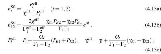
and with the corresponding Purcell rate $Q_1=4(g^\mathrm{eff})^2/\Gamma_2$ , the effective coupling strength at nonzero detuning $g^\mathrm{eff}=g/\sqrt{1+\Big(\frac{\Delta/2}{\Gamma_+} \Big)^2}$ and the phase $\phi=\arctan{(\frac{\Gamma_+}{\Delta/2})}$ . The only mean value that is missing to complete all SS nonvanishing ones is $n_\mathrm{B}$ , that takes a simple intuitive form in the SS,

$\displaystyle n_\mathrm{B}^\mathrm{SS}=\frac{n_1^\mathrm{SS}P_{E2}+n_2^\mathrm{SS}P_{E1}}{\Gamma_1+\Gamma_2}\leq n_1^\mathrm{SS}n_2^\mathrm{SS}\,.$

(4.15)

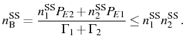
Note the difference with the equivalent $n_B^\mathrm{SS}$ for bosons, in Eq. (3.84), for which

$\displaystyle \langle\ud{a}a\ud{b}b\rangle^\mathrm{SS}\geq n_a^\mathrm{SS}n_b^\mathrm{SS}\,.$

(4.16)

This is an interesting manifestation of the symmetry/antisymmetry of the wavefunction for two bosons/fermions, that is known to produce such an attractive/repulsive character for the correlators.^4.1 Here we see that quantum (or correlated) probabilities $\langle n_1n_2\rangle$ (with

the number operator) are higher/smaller than classical (uncorrelated) probabilities $\langle n_1\rangle\langle n_2\rangle$ , depending on whether they are of a boson or fermion character, respectively. This provides a neat picture of bunching/antibunching from excitations of different modes that are otherwise of the same character. Mathematically, it is made possible from the fact that $\langle\ud{a}a\ud{b}b\rangle^\mathrm{SS}$ depends on other correlators of $\tilde{\mathcal{N}}_2$ , as we explained in Sec. 3.6, while $n_B^\mathrm{SS}$ does not (see Fig. 4.2).

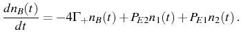
In the most general case, with pump and decay, from the initial to the steady state, also the transient dynamics of the mean values are given by the equivalent expressions from coupled bosons, Eq. (3.88). The general must be found by solving Eq. (4.12). 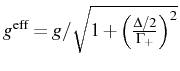We can conclude from this, as we did for the LM, that the single-time dynamics are ruled by the exact fermionic counterpart of the (half) Rabi frequency in Eq. (3.12), that we will refer to as $R^\mathrm{1TD}$ . In a naive approximation to the problem, following from the abundant similarities with the LM, one could imagine that the definitions of WC and SC regimes stem from the real part of $R_0^\mathrm{1TD}=R^\mathrm{1TD}(\Delta=0)$ , being zero or not. However, we will see that this is not the case whenever pump and decay are both taken into account. The single-time dynamics seems to disconnect completely from the more involved SC/WC distinction that we will find, solving the two-time dynamics.