

Steady State under continuous incoherent pumping
In the SS, at resonance,
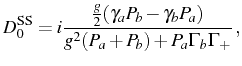
![]() is pure imaginary:
is pure imaginary:
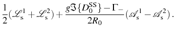
and the term that consists in the difference of Lorentzians in Eq. (3.37) disappears:
The only way to weight more one of the peaks than the other in the SS
of an incoherent pumping, would be to pump directly the polariton
(dressed) states, as is the case in higher-dimensional systems were
polaritons states with nonzero momentum relax into the ground state or
in 0D case when cross pumping is considered. In our present model,
however, such terms are excluded. The two peaks of the Rabi doublet,
composed of a Lorentzian and a dispersive part, are both symmetric
with respect to
![]() .
.
Only if
![]() , the spectrum of
Eq. (3.63) consists exclusively of two Lorentzians. The
parameters that correspond to this case are those fulfilling
either
, the spectrum of
Eq. (3.63) consists exclusively of two Lorentzians. The
parameters that correspond to this case are those fulfilling
either
![]() or
or
![]() . The second case corresponds to the limit of zero
broadening of the upper and lower branches, that narrow as we get into
a ``lasing'' region with diverging populations. Note that this
spectra, composed of Lorentzians only, is the same in the exciton or
photon channel of emission due to the invariance under the exchange
. The second case corresponds to the limit of zero
broadening of the upper and lower branches, that narrow as we get into
a ``lasing'' region with diverging populations. Note that this
spectra, composed of Lorentzians only, is the same in the exciton or
photon channel of emission due to the invariance under the exchange
![]() . In the most general case, the dispersive part
will contribute to the fine quantitative structure of the spectrum,
bringing closer or further apart the maxima and thus altering the
apparent magnitude of the Rabi splitting. In some extreme cases, as we
shall discuss, it even contrives to blur the resolution of the two
peaks and a single peak results, even though the modes split in
energy.
. In the most general case, the dispersive part
will contribute to the fine quantitative structure of the spectrum,
bringing closer or further apart the maxima and thus altering the
apparent magnitude of the Rabi splitting. In some extreme cases, as we
shall discuss, it even contrives to blur the resolution of the two
peaks and a single peak results, even though the modes split in
energy.
As for the weak coupling formula for the spectrum, it simplifies to:
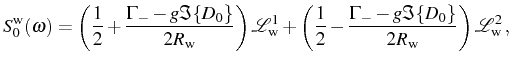
losing completely the dispersive contribution. Both decompositions, Eqs. (3.63) and (3.64), have been given to spell-out the structure of the spectra in both regimes. The unified expression that covers them both reads explicitly:
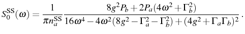
It is the counterpart for SS of Eq. (3.59), for SE. The case of excitonic emission can also be obtained, as for SE, exchanging the indexes
In order to study quantitatively the difference between the Rabi splitting of the dressed modes, given by
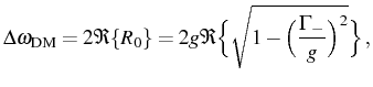
and the observed splitting, we solve Eq. (3.52). The symmetry of the resonant spectrum regarding the central frequency
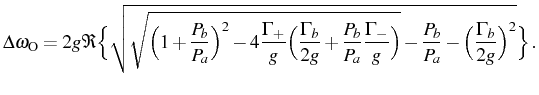
This simple expression can be straight forwardly used to estimate the system parameters from the experimental resonant lineshapes or to predict the pumping rates at which the splitting will be more visible for a given configuration. The counterpart expression for the splitting observed in the direct exciton emission can be obtained by simply exchanging indexes
The equivalent splitting in the SE emission is found by only
removing ![]() from the
from the ![]() 's and substituting
's and substituting ![]() by
the ratio of initial state populations
by
the ratio of initial state populations
![]() (under the
assumption that initially
(under the
assumption that initially
![]() , which ensures a symmetric
spectrum). In the case typically studied in the literature, that of
the spontaneous emission of an excited state (
, which ensures a symmetric
spectrum). In the case typically studied in the literature, that of
the spontaneous emission of an excited state (![]() and
and ![]() ),
we obtain the even simpler formulas
),
we obtain the even simpler formulas
 and
and
 for the splittings in the
cavity and direct exciton emission respectively, that were found by
Savona & (1995) or Cui & (2006).
for the splittings in the
cavity and direct exciton emission respectively, that were found by
Savona & (1995) or Cui & (2006).
![\includegraphics[width=\linewidth]{chap3/fig9-pyramids-spectra.eps}](img851.png) |
Elena del Valle ©2009-2010-2011-2012.