

Strong and Weak Coupling at resonance
Strong coupling is most marked at resonance, and this is where its
signature is experimentally ascertained, in the form of an
anticrossing. Fundamentally, there is another reason why resonance stands out as
predominant; this is where a criterion for SC can be
defined unambiguously in presence of dissipation:
WC and SC are formally defined as the regime where the complex
Rabi frequency at resonance, Eq. (3.33), is
pure imaginary (WC) or real (SC).
This definition, that takes into account dissipation and pumping,
generalizes the classification found in the literature. The reason for
this definition is mainly to be found in the behavior of the time
autocorrelator, Eq. (3.29), that is respectively damped or
oscillatory as a result. The exponential damping is the usual
manifestation of dissipation, that decays the correlations in the
field, even when a steady state is maintained. On the other hand, in
the same situation of steady averages (no dynamics) but now in SC,
oscillations with ![]() are the mark of a coherent exchange between
the bare fields (the photon field and exciton field).
are the mark of a coherent exchange between
the bare fields (the photon field and exciton field).
![\includegraphics[width=4.5cm]{chap3/newFigs/a.eps}](img782.png)
![\includegraphics[width=4cm]{chap3/newFigs/b.eps}](img783.png)
![\includegraphics[width=3.7cm]{chap3/newFigs/c.eps}](img784.png) |
![\includegraphics[width=0.45\linewidth]{chap3/fig6a-Init-spectra-ga_1.9-gb_0.1.eps}](img788.png)
![\includegraphics[width=0.45\linewidth]{chap3/fig6b-Init-dynamicsNa-ga_1.9-gb_0.1.eps}](img789.png) |
![\includegraphics[width=0.55\linewidth]{chap3/fig7a-Exciton-Init-spectra-ga_5.9-gb_0.1.eps}](img792.png)
![\includegraphics[width=0.55\linewidth]{chap3/fig7b-Photon-Init-spectra-ga_5.9-gb_0.1.eps}](img793.png)
![\includegraphics[width=0.55\linewidth]{chap3/fig7c-Init-dynamicsNa-ga_5.9-gb_0.1.eps}](img794.png) |
In the literature, one sometimes encounters the confusion that SC is
linked to a periodic transfer of energy or of population between the
photon and exciton field, or that it follows from a chain of emissions
and absorptions. This is an incorrect general association as one can
explicit cases with apparent oscillations of populations that
correspond to weak coupling, or on the contrary, cases with no
oscillations of populations that are in SC. The two concepts are
therefore logically unrelated in the sense that none implies the
other. This is illustrated for the SE case in
Figs. 3.5(a), 3.5(b)
and 3.6 on the one hand, where the system is in SC, and in
Fig. 3.5(c) and 3.7 on the
other hand, where it is in WC. In SS, there is no ![]() dynamics in any
case, so oscillations of populations are clearly unrelated to weak or
strong coupling. In SE, the distinction is clearly seen in
Fig. 3.5 where both the
dynamics in any
case, so oscillations of populations are clearly unrelated to weak or
strong coupling. In SE, the distinction is clearly seen in
Fig. 3.5 where both the ![]() and
and ![]() dynamics are shown in a contour-plot in the case where the system is
initially prepared as an exciton, (a) and (c), or as a polariton,
(b). In the polariton case, the dynamics in
dynamics are shown in a contour-plot in the case where the system is
initially prepared as an exciton, (a) and (c), or as a polariton,
(b). In the polariton case, the dynamics in ![]() is simply decaying
(because of the lifetime), while it is clearly oscillating in
is simply decaying
(because of the lifetime), while it is clearly oscillating in ![]() ,
were the proper manifestation of SC is to be found. The
,
were the proper manifestation of SC is to be found. The ![]() decay is
not exactly exponential because in the presence of dissipation, the
polariton is not anymore an ideal eigenstate (the larger the
dissipation, the more the departure). However this effect in SC is so
small that it only consists in a small ``wobbling'' of the
decay is
not exactly exponential because in the presence of dissipation, the
polariton is not anymore an ideal eigenstate (the larger the
dissipation, the more the departure). However this effect in SC is so
small that it only consists in a small ``wobbling'' of the ![]() contour lines. On the other hand, the exciton, (a), that is not an
eigenstate, features oscillations both in the
contour lines. On the other hand, the exciton, (a), that is not an
eigenstate, features oscillations both in the ![]() dynamics (the one
often but unduly regarded as the signature of SC), as well as
the
dynamics (the one
often but unduly regarded as the signature of SC), as well as
the ![]() dynamics. In stark contrast, the exciton in WC, (c),
bounces with
dynamics. In stark contrast, the exciton in WC, (c),
bounces with ![]() . This, that might appear as an oscillation, is not,
as it happens only once and is damped in the long-time values. This
behavior is shown quantitatively in Fig. 3.6 for SC and
Fig. 3.7 for WC, where the population
. This, that might appear as an oscillation, is not,
as it happens only once and is damped in the long-time values. This
behavior is shown quantitatively in Fig. 3.6 for SC and
Fig. 3.7 for WC, where the population ![]() is
displayed for the SE of an exciton (blue solid), a photon (purple
dashed) and an upper polariton (brown dotted), respectively, along
with the luminescence spectrum that they produce (detected in the
cavity emission). Here it is better seen how, for instance, the
polariton-decay is wobbling as a result of the dissipation, that
perturbs its eigenstate-character and leaks some population to the
lower polariton. More importantly, note how very different the
spectra are, depending on whether the initial state is a photon or an
exciton, despite the fact that the dynamics is similar in both cases
(see the inset in log-scale of their respective populations). The PL
spectrum observed in the cavity emission is much better resolved when
the system is initially in a photon state, than it is when the system
is initially in an exciton state. The splitting is larger and the
overlap of the peaks smaller in the former case. This will find an
important counterpart in the SS case. In Fig. 3.7, the
corresponding case of WC is shown for clarity, with a decay of
populations and possible oscillations.
is
displayed for the SE of an exciton (blue solid), a photon (purple
dashed) and an upper polariton (brown dotted), respectively, along
with the luminescence spectrum that they produce (detected in the
cavity emission). Here it is better seen how, for instance, the
polariton-decay is wobbling as a result of the dissipation, that
perturbs its eigenstate-character and leaks some population to the
lower polariton. More importantly, note how very different the
spectra are, depending on whether the initial state is a photon or an
exciton, despite the fact that the dynamics is similar in both cases
(see the inset in log-scale of their respective populations). The PL
spectrum observed in the cavity emission is much better resolved when
the system is initially in a photon state, than it is when the system
is initially in an exciton state. The splitting is larger and the
overlap of the peaks smaller in the former case. This will find an
important counterpart in the SS case. In Fig. 3.7, the
corresponding case of WC is shown for clarity, with a decay of
populations and possible oscillations.
![\includegraphics[width=0.66\linewidth]{chap3/fig8-CorrelatorSS-and-log-for-Points-on-pyr.eps}](img796.png) |
Figure 3.8 shows the ![]() dynamics in
the SS (when the
dynamics in
the SS (when the ![]() dynamics has converged and is steady), for five
cases of interest to be discussed later (in
Fig. 3.9). A first look at the dynamics
would seem to gather together a group of two curves that decay
exponentially to good approximation (and remain positive as a result),
and another group of three that assume a local minimum. The correct
classification is the most counter-intuitive in this regard, as it
puts together the dashed lines on the one hand and the solid on the
other. The mathematical reason for this classification is revealed in
the inset, where the same dynamics is plotted in log-scale. The dashed
(resp. solid) lines correspond to parameters where the system is in WC
(resp. SC) according to the definition, i.e., to values of
dynamics has converged and is steady), for five
cases of interest to be discussed later (in
Fig. 3.9). A first look at the dynamics
would seem to gather together a group of two curves that decay
exponentially to good approximation (and remain positive as a result),
and another group of three that assume a local minimum. The correct
classification is the most counter-intuitive in this regard, as it
puts together the dashed lines on the one hand and the solid on the
other. The mathematical reason for this classification is revealed in
the inset, where the same dynamics is plotted in log-scale. The dashed
(resp. solid) lines correspond to parameters where the system is in WC
(resp. SC) according to the definition, i.e., to values of ![]() that
are imaginary on the one hand and real on the other. In log-scale,
this corresponds respectively to a damping of the correlator, against
oscillations with an infinite number of local minima. Note that the
blue dashed line features one local minimum, which does not correspond
to an oscillatory--or coherent-exchange--behavior of the fields, but
rather to a jolt in the damping. These considerations that may appear
abstract at this level will later turn out to show up as the actual
emergence of split (dressed) states or not in the emitted spectrum.
that
are imaginary on the one hand and real on the other. In log-scale,
this corresponds respectively to a damping of the correlator, against
oscillations with an infinite number of local minima. Note that the
blue dashed line features one local minimum, which does not correspond
to an oscillatory--or coherent-exchange--behavior of the fields, but
rather to a jolt in the damping. These considerations that may appear
abstract at this level will later turn out to show up as the actual
emergence of split (dressed) states or not in the emitted spectrum.
We now return to the general (SE/SS) expression for the spectra, Eq. (3.37), that, at resonance in SC, simplifies to:
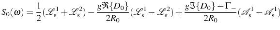
where we used the definition for the (half) Rabi frequency at resonance, Eq. (3.33), and
In the weak coupling regime, with ![]() pure imaginary
(
pure imaginary
(
![]() ), the positions of the two peaks collapse onto the
center,
), the positions of the two peaks collapse onto the
center,
![]() . Defining
. Defining
![]() , with
, with
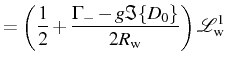
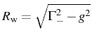 a real number, the general
expression for the spectra rewrites as:
a real number, the general
expression for the spectra rewrites as:
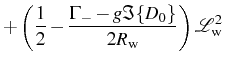
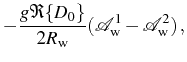
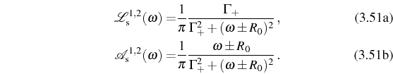
with the Lorentzian and dispersive contributions now given by:
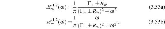
Before addressing the specifics of the SE and SS cases, it is
important to note that, at resonance, the Lorentzian and dispersive
parts [Eqs. (3.55) and (3.57)] are invariant
under the exchange of indexes
![]() . This is simply
because
. This is simply
because ![]() and
and ![]() are invariant under such
transformation. Therefore, the photon and the exciton spectrum are
composed of the same lineshapes, differing in the prefactor that
weights them in Eq. (3.54).
are invariant under such
transformation. Therefore, the photon and the exciton spectrum are
composed of the same lineshapes, differing in the prefactor that
weights them in Eq. (3.54).
Subsections Elena del Valle ©2009-2010-2011-2012.