

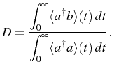
First order correlation function and power spectrum
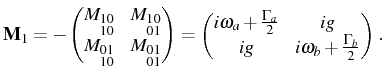
We now turn to the luminescence spectrum of the system ![]() given by Eq. (2.75). The equations for the two-time correlator
given by Eq. (2.75). The equations for the two-time correlator
![]() follow from the quantum regression
formula. The most general set of correlators we can construct is
follow from the quantum regression
formula. The most general set of correlators we can construct is
![]() , which satisfy
Eq. (2.98) for any operator
, which satisfy
Eq. (2.98) for any operator ![]() through the general regression matrix for the linear problem
given by:
through the general regression matrix for the linear problem
given by:
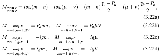
However in order to compute
and zero everywhere else. Furthermore, for the computation of the optical spectrum, it is enough to consider the subset
![\includegraphics[width=0.8\linewidth]{chap3/manifolds/FigNew-mani.ps}](img677.png) |
Thanks to the linearity of the problem, we obtain a simple equation,
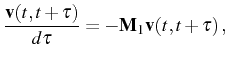
for the two-time correlators
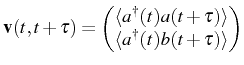
where
The formal solution follows straightforwardly from
![\begin{multline}
\langle\ud{a}(t){a}(t+\tau)\rangle =
e^{-\Gamma_+\tau}e^{-i...
...{(R-i\Gamma_-+\frac{\Delta}{2}) n_a(t) + g\,
n_{ab}(t)}{2R}\Big]
\end{multline}](img685.png)
with the complex (half) Rabi frequency that we defined in Eq. (3.12). The second correlator found together with Eq. (3.29) is the cross correlation function [defined in Eq. (2.83)] which here reads:
![\begin{multline}
\langle\ud{a}(t){b}(t+\tau)\rangle =
e^{-\Gamma_+\tau}e^{-i...
...R+i\Gamma_--\frac{\Delta}{2}) n_{abq}(t)-g\,
n_a(t)}{2R}\Big]\,.
\end{multline}](img686.png)
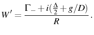
Before computing the spectrum of emission, let us look into the Rabi
frequency more in detail. Out of resonance, the Rabi frequency is a
complex number with both nonzero real,
![]() , and
imaginary,
, and
imaginary,
![]() , parts. The absolute value of these
frequencies can be written as:
, parts. The absolute value of these
frequencies can be written as:
For parameters
At resonance,
![\includegraphics[width=0.45\linewidth]{chap3/fig3a-Re-Rabi-detuning-decoherence.eps}](img697.png)
![\includegraphics[width=0.45\linewidth]{chap3/fig3b-Im-Rabi-detuning-decoherence.eps}](img698.png) |
The real and imaginary parts of ![]() are plotted in Fig. 3.3
as a function of
are plotted in Fig. 3.3
as a function of
![]() for various negative detunings. The
invariance of
for various negative detunings. The
invariance of ![]() under exchange of indexes
under exchange of indexes
![]() results in the property
results in the property
![]() . From
this follows the results of
. From
this follows the results of
![]() and
and
![]() for the
combinations of
for the
combinations of
![]() and
and ![]() that are not plotted in
the figure:
that are not plotted in
the figure:
In the limit of high detuning,
Once again, for the steady state case, we can obtain a range of
physical combinations of pumping intensities, ![]() ,
, ![]() , by ensuring
that the correlator of Eq. (3.29) converges to zero when
, by ensuring
that the correlator of Eq. (3.29) converges to zero when
![]() . Here, the condition follows from having a
positive total decay rate:
. Here, the condition follows from having a
positive total decay rate:
The first consequence of this condition is simply that
Using the result of Eq. (3.29) into the definition of Eq. (2.78), we obtain the formal structure of the emission spectrum:
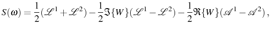
with
We also introduced the weight
that we define in terms of still another dimensionless parameter,
Written in this form, Eqs. (3.37)-(3.40) assume a
transparent physical meaning with a clear origin for each term. The
spectrum consists of two peaks (that we label 1 and 2), as is well
known qualitatively for the SC regime. These are composed of a
Lorentzian
![]() and a dispersive
and a dispersive
![]() part. We
already introduced the Lorentzian as the fundamental lineshape for
free particles with a lifetime, and in the expression above, it
inherits most of how the dissipation gets distributed in the coupled
system, including the so-called subnatural linewidth averaging
that sees the broadening at resonance below the cavity mode width, as
pointed out by Carmichael et al. (1989). The dispersive part originates
from the dissipative coupling as in the Lorentz (driven)
oscillator. It stems from the existence of resonant eigenenergies
(polaritons or dressed modes) in the system that overlap in energy and
interfere. The overlapping is due to decoherence that impedes the
Hamiltonian polaritons of Eq. (2.56) from
being the true eigenstates of the system. Also, which particles are
detected, in this case bare modes (photons or excitons), determines
greatly the dispersive contribution: the further the particles emitted
are from the eigenstates, the more relevant interference becomes. In
the case of very strong coupling, the Hamiltonian dynamics are the
most important and the dispersive part disappears. In the opposite
limit of WC, the dispersive part also disappears because the particles
emitted are those that rule the dynamics (photons or excitons)
although other kind of interference arises in the system, as we will
see, due to the coupling, weak, but still present.
part. We
already introduced the Lorentzian as the fundamental lineshape for
free particles with a lifetime, and in the expression above, it
inherits most of how the dissipation gets distributed in the coupled
system, including the so-called subnatural linewidth averaging
that sees the broadening at resonance below the cavity mode width, as
pointed out by Carmichael et al. (1989). The dispersive part originates
from the dissipative coupling as in the Lorentz (driven)
oscillator. It stems from the existence of resonant eigenenergies
(polaritons or dressed modes) in the system that overlap in energy and
interfere. The overlapping is due to decoherence that impedes the
Hamiltonian polaritons of Eq. (2.56) from
being the true eigenstates of the system. Also, which particles are
detected, in this case bare modes (photons or excitons), determines
greatly the dispersive contribution: the further the particles emitted
are from the eigenstates, the more relevant interference becomes. In
the case of very strong coupling, the Hamiltonian dynamics are the
most important and the dispersive part disappears. In the opposite
limit of WC, the dispersive part also disappears because the particles
emitted are those that rule the dynamics (photons or excitons)
although other kind of interference arises in the system, as we will
see, due to the coupling, weak, but still present.
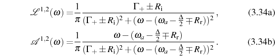
This decomposition of each peak in Lorentzian and dispersive parts is,
therefore, entirely clear and expected. More quantitatively, and
following the notation of our general expression for the spectra in
Eq. (2.105), the peaks, are placed at the
frequencies
![]() and have FWHM given by
and have FWHM given by
![]() . As
. As
![]() , the peaks
, the peaks ![]() and
and ![]() correspond
to the lower (``L'') and upper (``U'') branch emissions,
respectively. The weights are given by
correspond
to the lower (``L'') and upper (``U'') branch emissions,
respectively. The weights are given by
![]() and
and
![]() . The limit of bare modes at energies
. The limit of bare modes at energies
![]() and
and
![]() , broadened with the bare
parameters
, broadened with the bare
parameters
![]() (FWHM), is recovered at large detunings. The
bare cavity mode will be taken as a reference for the energy scales in
the rest of the Chapter (we set
(FWHM), is recovered at large detunings. The
bare cavity mode will be taken as a reference for the energy scales in
the rest of the Chapter (we set
![]() ). Again, we find that the
real (resp. imaginary) part of the complex Rabi frequency,
). Again, we find that the
real (resp. imaginary) part of the complex Rabi frequency,
![]() (
(
![]() ), contributes to the oscillations
(damping) in the correlator and therefore, to the positions
(broadenings) in the spectrum.
), contributes to the oscillations
(damping) in the correlator and therefore, to the positions
(broadenings) in the spectrum.
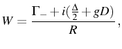
By defining new complex frequencies
the normalized and integrated first order correlation function can also be written, directly from Eq. (3.29), as:
The general expression for the spectrum in Eq. (3.37) therefore takes, thanks to the new parameters, the less physically meaningful but more compact form:
where
in terms of a parameter which is the counterpart of
Finally, the cross correlation spectral function that we defined in Eq. (2.84) reads:
So far, all the results hold for both cases of SE and SS. This shows that the qualitative depiction of SC is robust. This made it possible to pursue it in a given experimental system with the parameters of the theoretical models fit for another. This has indeed been the situation with semiconductor results explained in terms of the formalism built for atomic systems.
To be complete, the solution now only requires the boundary conditions
that are given by the quantum state of the system. They will affect
the parameter ![]() , Eq. (3.40), that is therefore the bridging
parameter between the two cases. In the next two sections, we address
the two cases and their specificities.
, Eq. (3.40), that is therefore the bridging
parameter between the two cases. In the next two sections, we address
the two cases and their specificities.
Subsections Elena del Valle ©2009-2010-2011-2012.