Overlay of a Mathematica plot with an image

Revision as of 12:13, 18 May 2020

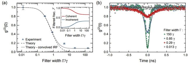
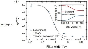
One often wants to compare a printed graph with one's own Mathematical curve. When the curve is fixed, I use Inkscape to do that, with opacity of either one of the images. That's the simplest. If the curve is varying, however, one can use Mathematica's Manipulate to do something similar, on the go. Here's an example that comes from a nice paper from Sheffield & Manchester on the Photon Statistics of Filtered Resonance Fluorescence, by Catherine Phillips et al. There, among other things, they checked the loss of antibunching in resonance fluorescence that we theorized in a series of papers. This is their Fig. 2:

Now in Ref. ^[1], we have a theoretical formula (Eq. (19b)) for what should be the theory curve on the left. In tidied-up notations, this is:

$$g^{(2)}(\tau=0)=\frac{\digamma_{11}\left(\gamma_\sigma ^2+4 \Omega ^2\right) \left(\digamma_{11}\digamma_{12}+8 \Omega ^2\right) \left(48 \Gamma ^2 \Omega ^4 \digamma_{21}+4 \Gamma \Omega ^2 \digamma_{31} \left(17 \Gamma ^3+29 \Gamma ^2 \gamma_\sigma +18 \Gamma \gamma_\sigma ^2+4 \gamma_\sigma ^3\right) +\digamma_{11}\digamma_{21}^2\digamma_{31}^2 \digamma_{12}\digamma_{32}\right)} {\digamma_{21}\digamma_{31}\left(\digamma_{11}\digamma_{21}+4 \Omega ^2\right) \left(\digamma_{31}\digamma_{32}+8 \Omega ^2\right) \left(\digamma_{12}\digamma_{11}^2 +4 \Gamma \Omega ^2\right)^2}$$

where we defined $\digamma_{kl}\equiv k\Gamma+l\gamma_\sigma$, for $\gamma_\sigma$ the radiative decay rate of the two-level system, $\Gamma$ the filter's bandwidth and $\Omega$ the driving strength. In fact we also studied the same problem from the experimental perspective with Lukas Hanschke from the TUM et al. and find similar things (with a better agreement). The point is, is this "similar" exactly the same? Is our analytical expression a perfect match to their theory curve? Our colleagues do not give a closed-form expression for this result and we can only surmise they got it numerically. How do the two compare?

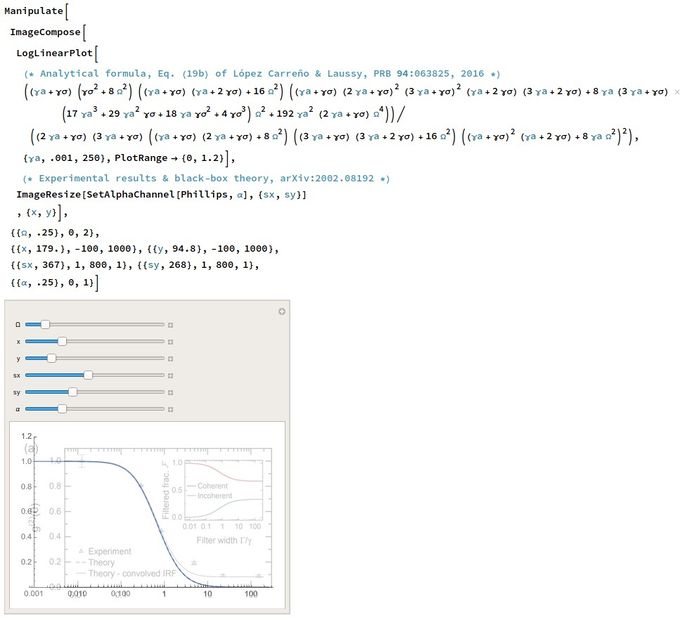
This is how to do it in Mathematica, combining ImageCompose, ImageResize & SetAlphaChannel:

The image is screenshot and pasted directly into the notebook & defined as something (here, Phillips, after the first author) and the following code that includes x and y to position horizontalwise & verticalwise the image, and sx, sy to scale it, so as to align it with the Mathematica plot, and α to change the transparency (opacity):

In code (you can copy/paste this in a notebook but you'll need to define the image):

Manipulate[
 ImageCompose[
  LogLinearPlot[
   (* Analytical formula, Eq. (19b) of López Carreño & Laussy, PRB 94:
   063825, 2016 *)
   ((\[Gamma]a + \[Gamma]\[Sigma]) (\[Gamma]\
\[Sigma]^2 + 
        8 \[CapitalOmega]^2) ((\[Gamma]a + \[Gamma]\[Sigma]) \
(\[Gamma]a + 2 \[Gamma]\[Sigma]) + 
        16 \[CapitalOmega]^2) ((\[Gamma]a + \[Gamma]\[Sigma]) (2 \
\[Gamma]a + \[Gamma]\[Sigma])^2 (3 \[Gamma]a + \[Gamma]\[Sigma])^2 (\
\[Gamma]a + 2 \[Gamma]\[Sigma]) (3 \[Gamma]a + 2 \[Gamma]\[Sigma]) + 
        8 \[Gamma]a (3 \[Gamma]a + \[Gamma]\[Sigma]) (17 \[Gamma]a^3 \
+ 29 \[Gamma]a^2 \[Gamma]\[Sigma] + 18 \[Gamma]a \[Gamma]\[Sigma]^2 + 
           4 \[Gamma]\[Sigma]^3) \[CapitalOmega]^2 + 
        192 \[Gamma]a^2 (2 \[Gamma]a + \[Gamma]\[Sigma]) \
\[CapitalOmega]^4))/((2 \[Gamma]a + \[Gamma]\[Sigma]) (3 \[Gamma]a + \
\[Gamma]\[Sigma]) ((\[Gamma]a + \[Gamma]\[Sigma]) (2 \[Gamma]a + \
\[Gamma]\[Sigma]) + 
        8 \[CapitalOmega]^2) ((3 \[Gamma]a + \[Gamma]\[Sigma]) (3 \
\[Gamma]a + 2 \[Gamma]\[Sigma]) + 
        16 \[CapitalOmega]^2) ((\[Gamma]a + \[Gamma]\[Sigma])^2 (\
\[Gamma]a + 2 \[Gamma]\[Sigma]) + 8 \[Gamma]a \[CapitalOmega]^2)^2),
   {\[Gamma]a, .001, 250}, PlotRange -> {0, 1.2}],
    (* Experimental results & black-box theory, arXiv:2002.08192 *)
  
  ImageResize[SetAlphaChannel[Phillips, \[Alpha]], {sx, sy}]
  , {x, y}],
 {{\[CapitalOmega], .25}, 0, 2}, {{x, 179.}, -100, 
  1000}, {{y, 94.8}, -100, 1000}, {{sx, 367}, 1, 800, 1}, {{sy, 268}, 
  1, 800, 1}, {{\[Alpha], .25}, 0, 1}]

For those who are interested in the Physics: it's a perfect match.

↑ Excitation with quantum light. I. Exciting a harmonic oscillator. J. C. López Carreño and F.P. Laussy in Phys. Rev. A 94:063825 (2016).

— Fabrice • 11:42, 18 May 2020

[lopezcarreno16a-1] Excitation with quantum light. I. Exciting a harmonic oscillator. J. C. López Carreño and F.P. Laussy in Phys. Rev. A 94:063825 (2016).

[1]

@@ Line 5: / Line 5: @@
 <center><wz tip="Phillips ''et al.'''s antibunching with filtering. We happen to have a formula for their curve on the left (the dashed one, without convolution).">[[File:Phillips-lantibu.jpg|650px]]</wz></center>
-Now in Ref. {{cite|lopezcarreno16a}}, we have a theoretical formula (Eq. (19b)) for what should be this curve. In tidied-up notations, this is:
+Now in Ref. {{cite|lopezcarreno16a}}, we have a theoretical formula (Eq. (19b)) for what should be the theory curve on the left. In tidied-up notations, this is:
 $$g^{(2)}(\tau=0)=\frac{\digamma_{11}\left(\gamma_\sigma ^2+4 \Omega ^2\right) \left(\digamma_{11}\digamma_{12}+8 \Omega ^2\right)
@@ Line 13: / Line 13: @@
      \left(\digamma_{12}\digamma_{11}^2 +4 \Gamma  \Omega ^2\right)^2}$$
-where we defined $\digamma_{kl}\equiv k\Gamma+l\gamma_\sigma$, for $\gamma_\sigma$ the radiative decay rate of the two-level system, $\Gamma$ the filter's bandwidth and $\Omega$ the driving strength.
+where we defined $\digamma_{kl}\equiv k\Gamma+l\gamma_\sigma$, for $\gamma_\sigma$ the radiative decay rate of the two-level system, $\Gamma$ the filter's bandwidth and $\Omega$ the driving strength. In fact we also studied the same problem from the experimental perspective with [[Lukas Hanschke]] from the [[TUM]] ''et al.'' and find similar things (with a better agreement). The point is, is this "similar" exactly the same? Is our analytical expression a perfect match to their theory curve? Our colleagues do not give a closed-form expression for this result and we can only surmise they got it numerically. How do the two compare?
-Now, our colleagues do not give a closed-form expression for this result and we can only surmise they got it numerically. Does it match, is it the exact theoretical expression or something slightly different, how does it compare?
 This is how to do it in [[Mathematica]], combining [https://reference.wolfram.com/language/ref/ImageCompose.html ImageCompose], [https://reference.wolfram.com/language/ref/ImageResize.html ImageResize] & [https://reference.wolfram.com/language/ref/SetAlphaChannel.html SetAlphaChannel]: